Monolithic FSI solver

A short introduction to the FSI models implemented in the FEM_Library

$\newcommand{\bm}[1]{\boldsymbol{\mathbf{#1}}} \newcommand{\bvec}[1]{\mathbf{#1}} \newcommand{\bx}{\mathbf{x}} \newcommand{\bd}{\mathbf{d}} \newcommand{\bv}{\dot{\mathbf{d}}} \newcommand{\ba}{\ddot{\mathbf{d}}} \newcommand{\bmw}{\mathbf{w}} \newcommand{\bmv}{\mathbf{v}} \newcommand{\Nh}{N_h} \newcommand{\bU}{\mathbf{U}} \newcommand{\bp}{\bvec{p}} \newcommand{\VV}{\mathbf{V}} \newcommand{\WW}{\mathbf{W}} \newcommand{\QQ}{\mathbf{Q}} \renewcommand{\AA}{\mathbf{A}} \newcommand{\BB}{\mathbf{B}} \newcommand{\CC}{\mathbf{B}} \newcommand{\EE}{\mathbf{E}} \newcommand{\FF}{\mathbf{F}} \newcommand{\FFi}{\mathbf{f}^i} \newcommand{\FFe}{\mathbf{f}^e} \newcommand{\GG}{\mathbf{G}} \newcommand{\CC}{\mathbf{C}} \newcommand{\MM}{\mathbf{M}} \newcommand{\XX}{\mathbf{X}} \newcommand{\KK}{\mathbf{K}} \newcommand{\UU}{\mathbf{U}} \newcommand{\II}{\mathbf{I}} \renewcommand{\SS}{\mathbf{S}} \newcommand{\HH}{\mathbf{H}} \newcommand{\DD}{\mathbf{D}} \newcommand{\NN}{\mathbf{N}} \newcommand{\bmg}{\mathbf{g}} \newcommand{\R}{\mathbb{R}} \newcommand{\JJ}{\mathbf{J}} \newcommand{\RR}{\mathbf{R}} \newcommand{\PP}{\mathbf{P}}$

Problem definition
Space and time discretization
References

Problem definition

The fluid-structure interaction (FSI) model that we consider here consists in a two-fields problem, where the incompressible Navier-Stokes equations written in the Arbitrary Lagrangian Eulerian (ALE) form are coupled with the nonlinear elastodynamics equation modeling the solid deformation. Because of the ALE approach we employ, a third non-physical geometry (or mesh motion) problem is introduced. The latter accounts for the fluid domain deformation, which in turn defines the ALE map.

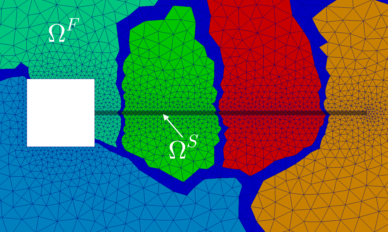
Let $\Omega^F$ and $\Omega^S$ be the domains occupied by the fluid and the solid in their reference configuration. We denote by $\Gamma = \partial \Omega^F \cap \partial \Omega^S$ the fluid-structure interface on the reference configuration. At any time $t$, the domain occupied by the fluid $\Omega^F(t)$ can be retrieved form $\Omega^F$ by the ALE mapping

$\begin{aligned} \mathcal{A}_t : \,\, &\Omega^F \rightarrow \Omega^F(t) \\ &\XX \mapsto \mathcal{A}_t(\XX) = \XX + \bd^G(\XX), \end{aligned}$

where $\bd^G$ represents the displacement of the fluid domain.

The coupled FSI problem thus consists in the following set of equations:

Navier-Stokes in ALE form governing the fluid problem: $$ \left\{ \begin{aligned} & \rho^F \frac{\partial \bmv^F}{\partial t}\Big|_{\XX} + (\bmv^F - \mathbf{w}^G) \cdot \nabla \bmv^F - \nabla \cdot \bm{\sigma}^F(\bmv^F, p^F) = \bm{0} & \text{ in } &\Omega^F(t) \\ &\nabla \cdot \bmv^F = 0 & \text{ in } &\Omega^F(t) \end{aligned} \right. $$ Nonlinear elastodynamics equation governing the solid dynamics: $$ \rho^S \frac{\partial^2 \mathbf{d}^S}{\partial t^2} \, - \nabla \cdot \PP(\mathbf{d}^S) = \mathbf{0} \quad \text{ in } \,\, \Omega^S $$ Coupling at the FS interface $\Gamma$: $$ \left\{ \begin{aligned} &\mathbf{v}^F = \frac{\partial \mathbf{d}^S}{\partial t} \\[5pt] &\bm{\sigma}^F(\bmv^F,p^F) \mathbf{n}^F + \bm{\sigma}^S(\mathbf{d}^S) \mathbf{n}^S = 0 \end{aligned} \right. $$ Linear elasticity equations modeling the mesh motion problem: $$ \left\{ \begin{aligned} & - \nabla \cdot \bm{\sigma}^G(\bd^G) = \mathbf{0} &\text{ in } & \Omega^F\\ & \mathbf{d}^G = \mathbf{d}^S \,\,\, &\text{on } &\Gamma \end{aligned} \right. $$

where $\bm{\sigma}^F(\bmv^F, p^F) = -p^F \mathbf{I} + 2 \mu^F \bm{\epsilon}(\bmv^F)$ is the fluid Cauchy stress tensor, $\bm{\sigma}^S(\mathbf{d}^S) = J^{-1} \PP \FF^T $ is the solid Cauchy stress tensor, and

$\bmw^G = \frac{\partial \bd^G}{\partial t}\Big|_{\XX}$

is the fluid mesh velocity. Both fluid and solid equations are complemented by appropriate initial and boundary conditions.

Space and time discretization

The field equations are discretized in space and time according to the following recipe:

We assume matching spatial discretizations between fluid and structure at the interface.
For the fluid velocity and pressure we use either $\mathbb{P}_2$-$\mathbb{P}_1$ finite elements or SUPG stabilized $\mathbb{P}_1$-$\mathbb{P}_1$ finite elements (see Bazilevs et al (2013) for the formulation of SUPG in the ALE setting); a BDF time-integrator is employed for the momentum equation.
The solid displacement is discretized using the same finite element space as for the fluid velocity; for the time integration, we use the Newmark scheme.
The fluid displacement is discretized using the same finite element space as for the fluid velocity.

As a result, we end up with a set of nonlinear algebraic equations for the residual forces in the interior of the geometry, fluid and solid fields

$\begin{equation} \begin{aligned} \RR^{F,n+1}_I(\bmv^{F,n+1}, p^{F,n+1}, \bd^{G,n+1}) & = \mathbf{0} \\ \RR^{S,n+1}_I(\bd^{S,n+1}) & = \mathbf{0} \\ \RR^{G,n+1}_I(\bd^{G,n+1}, \bd^{S,n+1}_\Gamma) & = \mathbf{0}. \end{aligned} \end{equation}$

The subscript $\Gamma$ at the structural displacement $\bd^{S,n+1}_\Gamma$ denotes the displacement restricted to the FSI interface. Equivalently, the subscript $I$ denotes system quantities from the respective field’s interior. At the the interface $\Gamma$ the equilibrium of stresses yields

$\begin{equation} \RR^{F,n+1}_\Gamma(\bmv^{F,n+1}, p^{F,n+1}, \bd^{G,n+1}) + \RR^{S,n+1}_\Gamma(\bd^{S,n+1}) = \mathbf{0}, \end{equation}$

while the discrete version of the kinematic coupling (continuity of the velocity) reads

$\begin{equation} \bmv_\Gamma^{F,n+1} = \bv_\Gamma^{S,n} + \frac{\gamma}{\beta \Delta t} \bd^{S,n+1}_\Gamma - \Delta t \gamma \bm{\xi}^{S,n}_{\Gamma} + \Delta t (1-\gamma) \ba^{S,n}_\Gamma. \label{eq:FSI11} \end{equation}$

Finally, the fluid domain deformation follows the structural displacement at the interface (geometric adherence)

$\begin{equation} \bd_\Gamma^{G,n+1} = \bd_\Gamma^{S,n+1}. \label{eq:FSI12} \end{equation}$

Combining equations \eqref{eq:FSI11} and \eqref{eq:FSI12}, we find that the fluid interface displacement follows form the fluid interface velocity:

$\bd^{G,n+1}_\Gamma = \bd^{S,n+1}_\Gamma = \frac{\beta \Delta t}{\gamma} \left( \bmv_\Gamma^{F,n+1} - \bv_\Gamma^{S,n} + \Delta t \gamma \bm{\xi}^{S,n}_{\Gamma} - \Delta t (1-\gamma) \ba^{S,n}_\Gamma \right).$

Newton method on the fully coupled system

To solve the nonlinear FSI problem applying the Newton method, the field residuals are combined to obtain the residual of the FSI problem (we drop the timestep superscript $n+1$ from now on)

$\begin{equation} \RR^{FSI} = \begin{pmatrix} \RR^{F}_I\\ \RR^{F}_\Gamma + \RR^{S}_\Gamma\\ \RR^{S}_I\\ \RR^{G}_I\\ \end{pmatrix} = \mathbf{0}. \end{equation}$

In the following, the fluid pressure variable $p^F$ is dropped from the notation, as it is understood that $\bmv^F$ represents all unknowns of the fluid field (with $p^F$ included in $\bmv^F_I$).

The Jacobian of the FSI residual (to be used within the Newton method) is derived in the following. To begin with, we denote by

$\FF = \frac{\partial \RR^F}{\partial \bmv^F}, \qquad \SS = \frac{\partial \RR^S}{\partial \bd^S}, \qquad \GG = \frac{\partial \RR^G}{\partial \bd^G},$

the Jacobians of the fluid, solid and geometry residuals with respect to fluid, solid and fluid displacement variables, respectively. Then, we introduce the linearization of the solid residual with respect to the fluid velocity

$\frac{\partial \RR^S}{\partial \bmv^F} = \frac{\partial \RR^S}{\partial \bd_\Gamma^S} \frac{\partial \bd_\Gamma^S}{\partial \bmv^F_\Gamma} = \begin{pmatrix} \frac{\partial \RR^S_I}{\partial \bmv^F} \\ \frac{\partial \RR^S_\Gamma}{\partial \bmv^F} \end{pmatrix} \frac{\partial \bd_\Gamma^S}{\partial \bmv^F_\Gamma} = \begin{pmatrix} \tau \SS_{I\Gamma} \\ \tau \SS_{\Gamma \Gamma} \end{pmatrix}$

where

$\tau = \frac{\partial \bd_\Gamma^S}{\partial \bmv^F_\Gamma} = \tfrac{\beta \Delta t}{\gamma}.$

Finally, we introduce the linearization of the fluid residual with respect to the mesh deformation, which yields the so-called shape derivatives

$\FF^G = \frac{\partial \RR^F}{\partial \bd^G}.$

The $k$-th step of the Newton scheme reads

$\begin{equation} \JJ^{FSI}(\bU^{n+1}_k) \, \delta \bU = -\RR^{FSI}(\bU^{n+1}_k), \label{eq:FSI20} \end{equation}$

where

$\bU = \begin{pmatrix} \bmv^F_I\\ \bmv^F_\Gamma\\ \bd^{S}_I\\ \bd^{G}_I\\ \end{pmatrix}$

is the vector of all unknowns, and the Jacobian matrix is given by

$\begin{equation} \JJ^{FSI} = \begin{pmatrix} \FF_{II} & \FF_{I\Gamma} + \tau \FF_{I\Gamma}^G & 0 & \FF_{II}^G\\ \FF_{\Gamma I} & \FF_{\Gamma \Gamma} + \tau \SS_{\Gamma \Gamma} + \tau \FF_{\Gamma \Gamma}^G & \SS_{\Gamma I} & \FF_{\Gamma I}^G\\ 0 & \tau \SS_{I \Gamma} & \SS_{II} & 0\\ 0 & \tau \GG_{I \Gamma} & 0 & \GG_{II} \end{pmatrix}. \label{eq:FSI21} \end{equation}$

Decoupling of the geometry problem

We note that omitting the shape derivatives $\FF^G$ decouples the geometry problem from the rest of the linear system \eqref{eq:FSI20}. Indeed, assuming that $\FF^G \approx 0$, the Jacobian matrix becomes

$\begin{equation} \JJ^{FSI} \approx \begin{pmatrix} \FF_{II} & \FF_{I\Gamma} & 0 & 0\\ \FF_{\Gamma I} & \FF_{\Gamma \Gamma} + \tau \SS_{\Gamma \Gamma} & \SS_{\Gamma I} & 0\\ 0 & \tau \SS_{I \Gamma} & \SS_{II} & 0\\ 0 & \tau \GG_{I \Gamma} & 0 & \GG_{II} \end{pmatrix}, \label{eq:FSI22} \end{equation}$

which reduces system \eqref{eq:FSI20} to the following

Fluid-Structure coupled problem: $$ \begin{equation} \begin{pmatrix} \FF_{II} & \FF_{I\Gamma} & 0 \\ \FF_{\Gamma I} & \FF_{\Gamma \Gamma} + \tau \SS_{\Gamma \Gamma} & \SS_{\Gamma I} \\ 0 & \tau \SS_{I \Gamma} & \SS_{II} \end{pmatrix} \begin{pmatrix} \delta \bmv_{I}^F \\ \delta \bmv_{\Gamma}^F \\ \delta \mathbf{d}_I^S\\ \end{pmatrix} \label{eq:FSI23} \end{equation} = - \begin{pmatrix} \RR^{F}_I\\ \RR^{F}_\Gamma + \RR^{S}_\Gamma\\ \RR^{S}_I\\ \end{pmatrix}. $$ Geometric problem: $$ \GG_{II} \mathbf{d}^G_I = - \GG_{I\Gamma} \mathbf{d}^S_{\Gamma}. $$

At each (quasi-)Newton iteration, this approach (that we refer to as monolithic fully-implicit) requires to:

assemble $\RR^F$ and $\FF$ on the deformed fluid mesh
assemble $\RR^S$ and $\SS$ on the undeformed solid mesh
form and solve system \eqref{eq:FSI23}
update the solution
solve the mesh motion (geometric) problem
move the mesh

Note that the matrix $\GG_{II}$ is assembled and factorized once and for all at the beginning of the simulation, thus leading to significant computational savings. This approach is often referred to as quasi-direct coupling, see e.g. Bazilevs et al (2013) and references therein.

Monolithic Geometry–Convective Explicit Scheme

With the aim of decreasing the computational costs entailed by the monolithic fully-implicit scheme, we introduce the so-called Monolithic Geometry–Convective Explicit (GCE) scheme. The latter is easily obtained by:

linearizing the fluid convective term using a BDF extrapolation as already described here;
treating the geometry problem explicitly.

We refer to Crosetto et al (2011) for further details.

Preconditioner

At each time step, the coupled linear system \eqref{eq:FSI23} is solved monolithically by means of either a direct or an iterative solver. In the latter case, we employ the GMRES with a one-level additive Schwarz (AS) preconditioner that preconditions the entire system together, following the approach proposed in Barker and Cai (2010), Wu and Cai (2014).

To this end, we generate a decomposition of the mesh which is completely independent of the physical variables defined at a given mesh point. As a result, a subdomain may contain both fluid and solid elements.

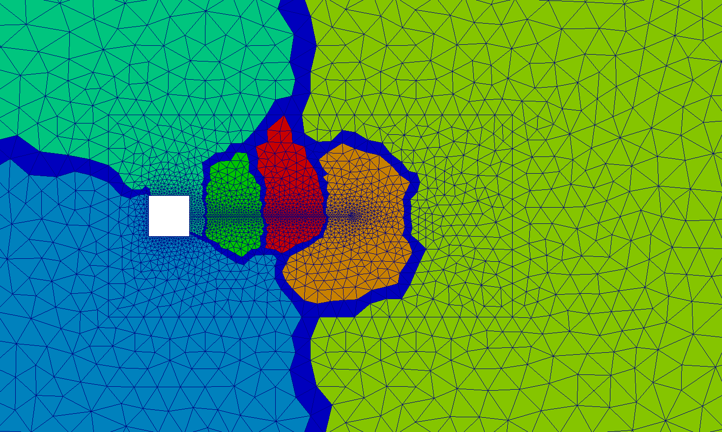
To build the AS preconditioner for the Jacobian matrix, we first partition the domain $\Omega = \Omega^F \cap \Omega^S$ into overlapping subdomains $\Omega_k^\delta$, $k=1\dots,K$, featuring an overlap of size $\delta \geq h$. We then build suitable restriction matrices $\RR_k \in \mathbb{R}^{\Nh^k \times \Nh}$ so that the local matrices $\JJ_k = \RR_k \JJ \RR_k^T \in \mathbb{R}^{\Nh^k \times \Nh^k}$ correspond to the restriction of $\JJ \in \R^{\Nh \times Nh}$ to the subdomains $\Omega_k^\delta$. The AS preconditioner is then defined as

$\PP^{-1}_{AS} = \sum_{k=1}^{K} \RR_k^T \JJ_k^{-1} \RR_k,$

$\JJ_k^{-1}$ being the inverse of $\JJ_k$, here computed by means of an exact LU factorization; each local preconditioner is then applied in parallel.

References

Y. Bazilevs, K. Takizawa, and T. E. Tezduyar. Computational fluid-structure interaction: methods and applications. John Wiley & Sons, 2013.
P. Crosetto, S. Deparis, G. Fourestey, and A. Quarteroni. Parallel algorithms for fluid-structure interaction problems in haemodynamics. SIAM Journal on Scientific Computing, 33(4):1598-1622, 2011.
M. W. Gee, U. Küttler, and W. A. Wall. Truly monolithic algebraic multigrid for fluid–structure interaction. International Journal for Numerical Methods in Engineering 85(8):987-1016, 2011.
D. Forti. Parallel Algorithms for the Solution of Large-Scale Fluid-Structure Interaction Problems in Hemodynamics. PhD thesis, EPFL, Lausanne, 2016.

Solid-extension mesh motion technique:

Stein, K., Tezduyar, T., Benney, R.: Mesh moving techniques for fluid-structure interactions with large displacements. J. Appl. Mech. 70(1), 58–63 (2003).
Stein, K., Tezduyar, T., Benney, R.: Automatic mesh update with the solid-extension mesh moving technique. Comput. Meth. Appl. Mech. Engrg. 193(21), 2019–2032 (2004).

Preconditioner:

A.T. Barker and X.C. Cai. Scalable parallel methods for monolithic coupling in fluid-structure interaction with application to blood flow modeling. J. Comput. Phys., 229(3):642–659, 2010.
Y. Wu and X.C. Cai. A fully implicit domain decomposition based ALE framework for three-dimensional fluid-structure interaction with application in blood flow computation. J. Comput. Phys., 258:524–537, 2014.